
This is the third post in the tidy sports analytics series. In this series, I’ve been demonstrating how the collection of tidyverse packages can be used to explore and analyze sports data. Specifically, I’ve been using the 2016 NFL play-by-play data from Armchair Analysis. Part one in the series showed how dplyr can be used for data manipulation, and part two demonstrated reshaping and tidying data using tidyr. This post focuses on data visualization using ggplot2.
ggplot2
Data visualization is a key part to any data or sports analytics analysis. In the tidyverse, visualization is mainly handled through ggplot2. There is an ongoing debate in the R community as to whether base graphics or ggplot2 should be used (see here, here, and here). In practice, you should use whichever tools are going to be effective. Both sets of tools will be able to solve a wide variety of visualization issues, just in different ways. Given that this series of blog posts is focused on using the tidyverse, it’s probably obvious that I prefer ggplot2. But rather than try to compare and contrast these two systems, I’m going to point out a few features that I think make ggplot2 particularly appealing as I demonstrate how it can be used to visualize sports analytics data.
ggplot2 is built around the idea of a grammar of graphics. That is, rather than having a typology of visualizations (e.g., scatter plot, bar plot, histogram, etc.), the grammar of graphics focuses on on the individual pieces of a plot. A visualization is created by assembling your various graphical parameters. ggplot2 works by mapping the data to different aesthetics in the plot, and then adding graphical elements, or geoms.
Using ggplot2
First, let’s get our data to the point where it was at the end of the previous post.
library(tidyverse)

success <- read_rds("data/nfl_pbp_2016.rds") %>%
  select(game_id = gid, play_id = pid, offense = off, defense = def,
         play_type = type, down = dwn, to_go = ytg, gained = yds) %>%
  filter(play_type %in% c("PASS", "RUSH")) %>%
  mutate(
    needed = case_when(
      down == 1 ~ to_go * 0.45,
      down == 2 ~ to_go * 0.60,
      TRUE ~ to_go * 1.00
    ),
    play_success = case_when(
      gained >= needed ~ TRUE,
      gained < needed ~ FALSE
    )
  ) %>%
  gather(key = "team_unit", value = "team", offense:defense) %>%
  mutate(
    play_success = case_when(
      team_unit == "defense" ~ !play_success,
      TRUE ~ play_success
    )
  ) %>%
  group_by(team, team_unit) %>%
  summarize(success_rate = mean(play_success, na.rm = TRUE)) %>%
  spread(key = team_unit, value = success_rate) %>%
  ungroup()
success
#> # A tibble: 32 × 3
#>    team  defense offense
#>    <chr>   <dbl>   <dbl>
#>  1 ARI     0.579   0.458
#>  2 ATL     0.512   0.500
#>  3 BAL     0.580   0.410
#>  4 BUF     0.553   0.464
#>  5 CAR     0.542   0.420
#>  6 CHI     0.550   0.461
#>  7 CIN     0.558   0.464
#>  8 CLE     0.546   0.409
#>  9 DAL     0.521   0.511
#> 10 DEN     0.594   0.423
#> # … with 22 more rows
The first plot we can make is a scatter plot of offensive success rate vs. defensive success rate.
ggplot(data = success, mapping = aes(x = defense, y = offense)) +
  geom_point()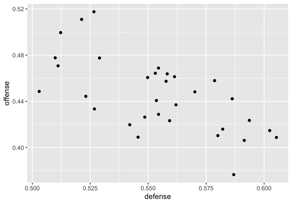
Figure 1: Basic scatterplot
Here, we define the data that will be used for the plot, then define how the variables in the data map to the plot. Specifically, we want defensive success rate on the x-axis, and offensive success rate on the y-axis. Finally, we use geom_point to add points at each of (x, y) coordinates defined in the aesthetic mapping. In Figure 1 each point represents a team. The x-axis represents the percent of plays that each teams’ defense was successful, and the y-axis represents the percent of play that each teams’ offense was successful. It appears that there is a general trend of a more successful defense being associated with a less successful offense. We can look at this trend by using geom_smooth. This function will calculate a line of best fit for the data using the method of our choice.
ggplot(data = success, mapping = aes(x = defense, y = offense)) +
  geom_point() +
  geom_smooth(method = "lm")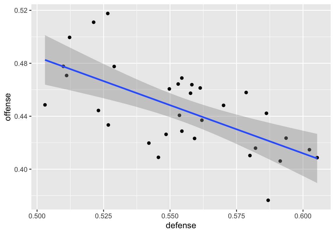
Figure 2: Scatterplot with linear best fit line
With ggplot, it’s easy to add extra elements to customize the specific pieces needed for the visualization. Each geom also comes with its own options. For example, in geom_smooth, we’ve specified the "lm" smoothing method. By default, geom_smooth will create a loess line; however, here we used "lm" to create a line based on a linear regression model. Therefore, the line is linear, rather than a line that fluctuates. We can also specify groupings in the plots. Just as groupings allowed us to make calculations by group in the previous post, groupings in ggplot2 allow us to map certain aesthetics at the group level. For example, we can map different colors to each group. For effective grouping, the data will need to be in long format, which can be accomplished using the gather function. A more detailed example and explanation of using the gather function can be found in part two.
success <- gather(success, key = "team_unit", value = "success_rate",
  defense:offense)
success
#> # A tibble: 64 × 3
#>    team  team_unit success_rate
#>    <chr> <chr>            <dbl>
#>  1 ARI   defense          0.579
#>  2 ATL   defense          0.512
#>  3 BAL   defense          0.580
#>  4 BUF   defense          0.553
#>  5 CAR   defense          0.542
#>  6 CHI   defense          0.550
#>  7 CIN   defense          0.558
#>  8 CLE   defense          0.546
#>  9 DAL   defense          0.521
#> 10 DEN   defense          0.594
#> # … with 54 more rows
Figure 3 shows how we can make a grouped bar plot. First, we filter the data to only include teams in the AFC West. This limits the number of teams that will need to be displayed on the x-axis. The success_rate is then mapped to the y-axis, and we specify that we want the fill of the bar to correspond to the offense and defense. Thus, for each team, their offensive success rate will be one color, and their defensive success rate will be another. Finally, geom_col is uses to make the bars. By default, stacked bars are created, but specifying position = "dodge" instead tells ggplot2 to group them side by side. Notice that ggplot2 will automatically create the legend for you.
ggplot(data = filter(success, team %in% c("DEN", "KC", "OAK", "SD")),
       mapping = aes(x = team, y = success_rate, fill = team_unit)) +
  geom_col(position = "dodge") +
  scale_fill_discrete(name = "Team Unit") +
  labs(x = NULL, y = "Success Rate")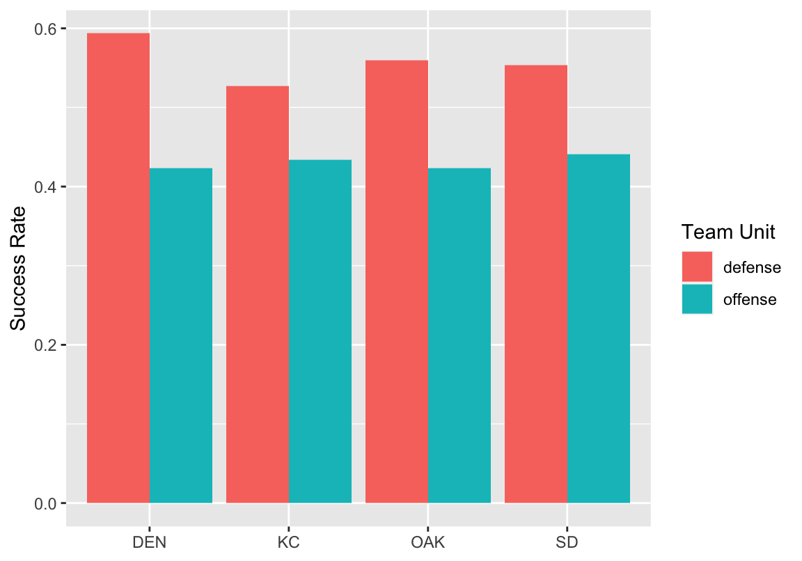
Figure 3: AFC West success rates
There is an almost endless series of geoms that can be combined to make your desired visualization. Everything in these plots can be customized: colors, titles and labels (as was done in Figure 3), and even fonts can be changed. However, this goes beyond the scope of this post. Instead, I wanted to show easy it can be to use ggplot2 to create professional looking graphics. Creating professional graphics can go a long way in people taking your work seriously. I have found that often, people I’m making presentations to go straight to the graphics because they are eye catching. Thus it is important for the graphics to look professional. Because of this it is also important for graphics to be able to stand alone and provide all of the necessary information. With ggplot2, legends are created automatically and it is easy to modify axes and their labels. Thus, this is a much more straight forward process than in other R graphics systems.
Conclusion
The ggplot2 package is a powerful tool for data visualization. Here, I’ve provided a brief introduction to the package’s mechanics. Once you’ve mastered the basics, it becomes much simpler to create more complex graphics. Because of the grammar of graphics, the creation of plots can be reduced to two steps: 1. select relevant geoms, and 2. map the data to the necessary aesthetics. In the next and final post in this series, I’ll pull everything together, talk about the tidyverse more generally, and describe some of the other benefits associated with its use. For more ggplot2 resources, check out:
Acknowledgments
Featured photo by Melissa McGovern on Unsplash.