
The Big 12/SEC challenge tips off tomorrow. This will be the 4th year of this competition, and the Big 12 has never lost. In this post, we’ll use a Monte Carlo simulation to estimate the Big 12’s chances of continuing this streak for another year.
As always, the code and data for this post are available on my Github page.
The Ratings
The team ratings are composite ratings, based off of Elo ratings and adjusted efficiencies. We first have to adjust these ratings for home court advantage1, and then we can calculate the probability that the Big 12 will win each game using the Log-5 formula.
library(dplyr)
library(ggplot2)
library(purrr)
library(readr)

big12sec <- read_csv("data/big12sec_2017.csv",
  col_types = "ccn")
big12sec
#> # A tibble: 10 x 3
#>    Home            Away            Big12_Win
#>    <chr>           <chr>               <dbl>
#>  1 West Virginia   Texas A&M           0.944
#>  2 Oklahoma        Florida             0.287
#>  3 Tennessee       Kansas State        0.490
#>  4 Texas Tech      Louisiana State     0.912
#>  5 Georgia         Texas               0.335
#>  6 Vanderbilt      Iowa State          0.658
#>  7 Oklahoma State  Arkansas            0.737
#>  8 Kentucky        Kansas              0.282
#>  9 Mississippi     Baylor              0.843
#> 10 Texas Christian Auburn              0.839
After accounting for the location of each game, we can see, for example, that Kansas has around a 28% chance of beating Kentucky, and Oklahoma State has a 74% chance of beating Arkansas. To get the expected number of wins for the Big 12, we can sum the probabilities of the Big 12 winning each game. Doing this, we get an expected number of wins of 6.33. This means that if we repeated the Big 12/SEC challenge multiple times, on average, the Big 12 would get about 6.33 wins.
Monte Carlo Simulation
It’s not possible for us to repeat the Big 12/SEC challenge multiple times in real life, but we can do this through a process called Monte Carlo simulation. In a Monte Carlo simulation we can generate data for an event multiple times, and then average the results over all replications. To illustrate, we can simulate the winner of the Kansas vs. Kentucky game. According to the model, Kansas has a 28% chance of winning. We generate a random number between 0 and 1. If that number is less than 0.28, then Kansas is the winner of the simulation, otherwise, Kentucky is the winner. We do this for every game, and then count the number of winners that come from the Big 12 to determine which conference won the challenge (or if it was a tie). We then repeat this process over and over again to simulate many replications of the challenge.
To enact this process in R, we’ll first need to define some functions. The first function will take in the probability of a team winning (in our case the Big 12 team), and return a 1 if that team wins, and a 0 otherwise.
sim_game <- function(prob) {
  ifelse(runif(1, min = 0, max = 1) < prob, 1, 0)
}
We can then define a function that takes in a vector of probabilities, and returns the number of wins.
sim_challenge <- function(prob_vec) {
  map_dbl(.x = prob_vec, .f = sim_game) %>% sum()
}
Finally, we can use the purrr package to simulate the Big 12/SEC challenge 10,000 times. Importantly, we need to set the random seed generator in order to make this analysis replicable.
set.seed(71715)
num_sim <- 10000

challenge_wins <- map_dbl(.x = seq_len(num_sim), .f = function(x, prob_vec) {
  sim_challenge(prob_vec)
}, prob_vec = big12sec$Big12_Win)

sim_results <- data_frame(big12_wins = challenge_wins) %>%
  group_by(big12_wins) %>%
  summarize(n = n())
sim_results
#> # A tibble: 10 x 2
#>    big12_wins     n
#>         <dbl> <int>
#>  1          1     1
#>  2          2    12
#>  3          3   158
#>  4          4   626
#>  5          5  1785
#>  6          6  2878
#>  7          7  2755
#>  8          8  1380
#>  9          9   367
#> 10         10    38
As we would expect, the most common outcome was the Big 12 winning 6 games. This occured 2,878 times. The second most common outcome was the Big 12 winning 7 games, which occured 2,755 times. Also note that although there were 38 simulations where the Big 12 went undefeated, there no simulations where the Big 12 failed to win a game, and only 1 simulation where the Big 12 won a single game.
Plotting the Results
Now that we have a distribution for the number of wins for the Big 12, we can plot the distribution using ggplot2. First we assign a conference winner to each number of wins.
sim_results$winner <- case_when(
  sim_results$big12_wins < 5 ~ "SEC",
  sim_results$big12_wins > 5 ~ "Big 12",
  TRUE ~ "Tie"
)
sim_results
#> # A tibble: 10 x 3
#>    big12_wins     n winner
#>         <dbl> <int> <chr>
#>  1          1     1 SEC
#>  2          2    12 SEC
#>  3          3   158 SEC
#>  4          4   626 SEC
#>  5          5  1785 Tie
#>  6          6  2878 Big 12
#>  7          7  2755 Big 12
#>  8          8  1380 Big 12
#>  9          9   367 Big 12
#> 10         10    38 Big 12
Then we can calulate the probability of each outcome.
outcome <- sim_results %>%
  group_by(winner) %>%
  summarize(probability = sum(n) / num_sim) %>%
  mutate(probability = paste0(sprintf("%0.1f", probability * 100), "%"))
outcome
#> # A tibble: 3 x 2
#>   winner probability
#>   <chr>  <chr>
#> 1 Big 12 74.2%
#> 2 SEC    8.0%
#> 3 Tie    17.8%
Finally, we put all of that information together and plot the distribution!
sim_results %>%
  mutate(n = n / num_sim) %>%
  ggplot(aes(x = factor(big12_wins, levels = 0:10), y = n, fill = winner)) +
  geom_col() +
  scale_x_discrete(drop = FALSE) +
  scale_y_continuous(breaks = seq(0, 1, 0.1),
    labels = paste0(seq(0, 100, 10), "%")) +
  scale_fill_brewer(name = "Winner", type = "qual", palette = 7) +
  labs(title = "Big 12/SEC Challenge Probabilities",
    subtitle = paste(paste0(outcome$winner, ": ", outcome$probability),
      collapse = "  |  "), x = "Big 12 Wins", y = "Probability") +
  theme_minimal() +
  theme(legend.position = "bottom") +
  guides(fill = guide_legend(title.position = "top", title.hjust = 0.5))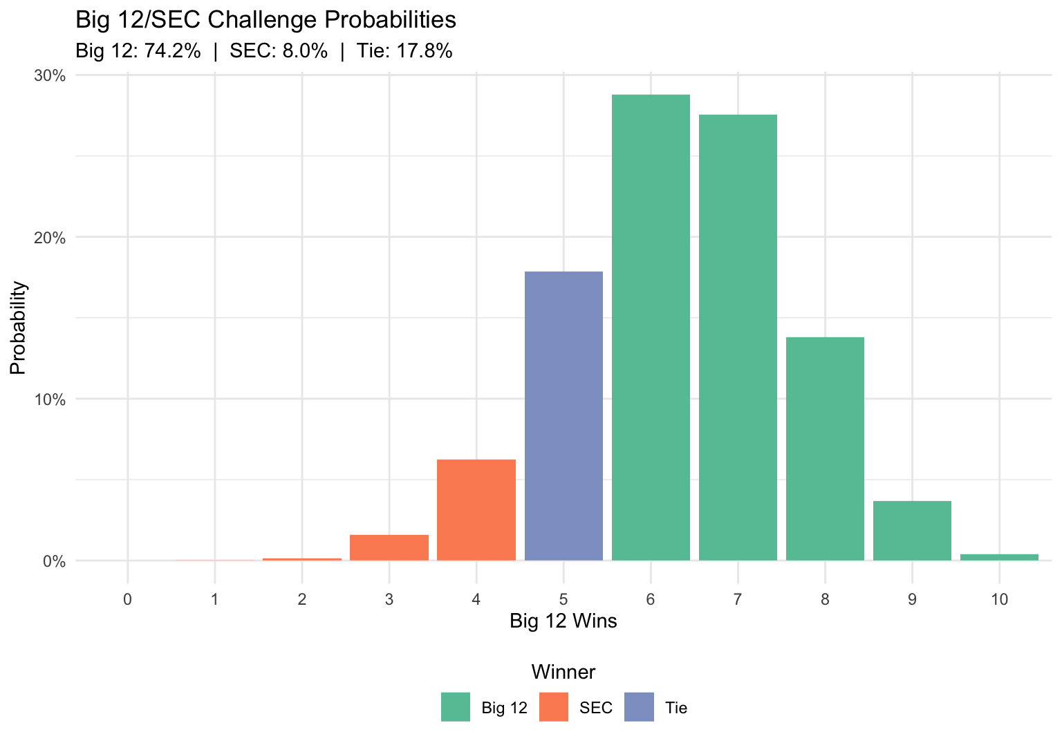
Conclusion
The results of the simulation show that the Big 12 has about a 74% chance of winning the challenge and continuing their streak. I’ll be tweeting out updated probabilities throughout the day tomorrow as the games finish, so follow me there for updates!
Acknowledgments
Featured photo by Danny Lines on Unsplash.
Footnotes
The home team’s offense is increased by 30% and defense is decreased by 30%, and the reverse is done for the away team.↩︎